- Why R with TensorFlow
- Deep learning neural networks
- Environment setup
- TensorFlow
- Keras
- Example project
- Conclusion
Code repo: https://github.com/mirano-galijasevic/DeepLearning/blob/master/AdultCensusClassifier.r
WHY R WITH TENSORFLOW
I am a big proponent of using the R-Studio for Machine Learning, as it offers the superb environment where you are in a driving seat and can do even most complicated tasks with a relative ease. Now with the packages for TensorFlow it has become even more powerful.
This post aim at providing an introductory information on what the deep neural networks are good for, and how the R and TensorFlow can be used in this respect. Since I am a firm believer in providing just enough theory so that the concepts can be understood and then moving on with a real-world scenario, this is the way we will do it here as well. The focus of this post is to provide you with a basic info on how to use RStudio, R, TensorFlow, deep neural networks and Keras for a simple machine learning project.
It would be good if you were somewhat familiar with neural networks and basic machine learning concepts, such as using regression, classification and clustering at a basic level. Also, understanding Algebra is a must for any work in artificial intelligence, namely linear equations, functions and graphs, vectors and matrices and basic probability and statistical functions. Knowing Calculus topics, such as Limits, Derivates and Integrals would be a huge plus. Tooling today is so advanced and libraries that exist are so powerful, that you really do not need to be proficient in Math to run machine learning experiments, but if you really want to understand what is going on and not just run automated tasks with 99% of the work being done by some packages, then you should really have a good understanding of the underlying mathematical theory.
The Artificial Intelligence is a big topic these days, and more so with several dystopian scenarios where machines take over everything and we are erased as living beings, or in the best scenario they decide to keep us as pets. Anybody who understands today’s technological level of AI will find this amusing, since AI is nowhere near that level that it can connect to human brain, exchange the information with it directly without any interface, or download the whole brain to a cloud, as it was suggested. I guess this is all entertaining for many people, so they keep on coming up with these grim forecasts, like Elon Musk of Tesla and SpaceX ( https://cnb.cx/359XwX0 ), Ray Kurzweil, Google’s director of Engineering ( https://bit.ly/3bJ6ME9 ) or David Icke ( https://bit.ly/2W2jkjm ).
Apart from being amusing, I do not find too much merit in these views, since the “intelligent” bit in deep learning networks is really down to mathematical functions that “learn” by using some kind of a loss function that automatically optimizes the parameters, and then runs the transformation functions over and over again until the model is trained sufficiently. There is really nothing akin human-like “thinking” there, and we should not even start with things like feelings, deep intuition, inspiration or such. So it is all very technical and firmly rooted in mathematics, and reminds me a little bit of a period in the dawn of the industrial revolution when people would smash the machines as they would perceive them as being a threat to their jobs and lives. This is now a similar situation, just the machine learning algorithms are getting better and better, with the big data in clouds so that we have the data samples that were unthinkable of before and that we can train the models on, but again it just boils down to sophisticated mathematical operations that can solve complex logical and other more fuzzy-like challenges that may appear to be produced by a thinking machine, which is really not the case. To conclude, I see no reason for all this fuss and bad publicity, but we should instead focus on all the good it brings. For that matter, let us leave the philosophical aspects of AI to the philosophers, and all the skewed reality to the imagination of film makers to create something fun to watch, even though not rooted in any real science. Later in this post we’ll get into the mechanics on how these networks and layers work in order to at least conceptually understand it in a more generalized way, but for now let us first get oriented what role deep learning plays in today’s field of the AI. We can represent this relationship with the figure 1.1. below:

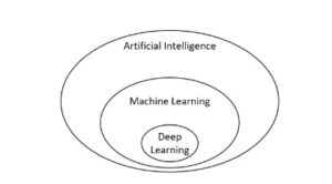 Figure 1.0: AI, Machine Learning and Deep Learning
In the overall field of AI, the first attempts to solve logical problems was made with symbolic programming, then it improved and grew into the machine learning in order to solve other not so well-defined logical challenges. Now we have a further specialization of machine learning in Deep Learning networks, which achieve their result by implementing many layers of data transformation in order to train the models well. Deep learning heavily relies on the existence of big data and employing it on relatively small data sample is likely not to achieve better results than the standard machine learning algorithms.
To understand what it does and how it defers from the machine learning, we first need to understand how the machine learning is different than regular programming. The simplest way to put it is to understand that machine learning is an attempt to not use the regular programming where we have certain rules coded in some programming language and then they operate on some input data and provide the output, but the machine learning instead is trying to analyze data and sort of understand the connections and relations in the data, and comes up with the set of rules itself. This may seem simple enough, and it is, but applied correctly it can solve many intellectual challenges in real life.
Now deep learning is an additional improvement on machine learning algorithms where it used the models that are usually represented as neural networks and then applies transformations with many layer, possibly hundreds of them, in order to make better and better representations that all improve the model in each successive run. Not going too deep down the rabbit hole, it is still beneficial that we understand what is under the hood, at least conceptually. Let us consider the following model:
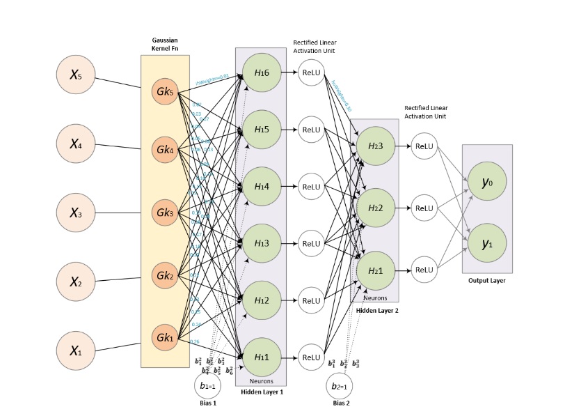
Figure 1.1: Deep Learning Neural Network
If the deep neural network in Figure 1.1. reminds you of a feed-forward neural network, that is because it is a feed-forward network with many hidden layers.
As shown in figure 1.1, the inputs are fed into the neural network which consists of many layers, often several hundreds, and the output is shown on the right-hand side. So the processing flows between multiple layers, and the actual learning occurs in the loss function that is used to calculate the output that is used to improve the learning, and then the optimizer is deciding on how it will incorporate that result in the proceeding. Going forwarder between these layers is called forwardpropagation, and going back is called backpropagation.
We are going to use one or more tensors as input into the network (more on tensors later when we introduce the TensorFlow, for now just think of tensors as various shaped arrays and matrices), and they will be processed by neural networks from Keras library (more on that later as well). Suffice to say that Keras library helps with implementing various, often very complicated neural networks, as it offers more than 60 typical neural networks, plus others that you can define yourself. In general, we create deep neural networks by combining the compatible neural networks into sort of a pipeline for processing and transforming the input data.
When I say compatible, it really means that not every neural network can accept any type of data. For instance, if we have a standard two-dimensional data in the form of a matrix:


then we are creating a two-dimensional matrix with 3 rows, 3 columns, and filling it in with number 11, so something like this:

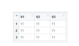
Now, we process this kind of data with dense or fully connected layers from Keras. On the other hand, if we have image data, stored in 4D tensors, then we use convolutional layers for processing, and so on, you get the idea. It is important to just understand that certain shape of data used as inputs should be processed by certain types of layers, and those layers then output the data in a specific shape again. As we shall see, Keras is a great library that helps us a lot to provide the proper shape of data to the next layer by being very smart in inferring the data shapes, but more on that later.
Back to the Figure 1.1., the key part of the deep neural networks are loss functions
and optimizers used to determine how the success determined in the loss function should be used to update the network. It usually uses stochastic gradient descent algorithm to do the work. Loss function and optimizers are the heart of the process, so we should examine them more carefully. The whole process looks like a pipeline that runs something like this:

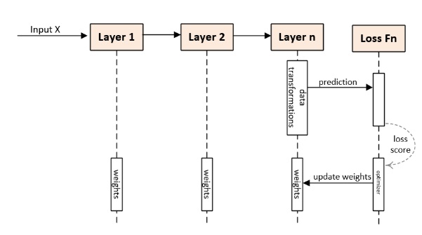
Loss Function – as seen in Figure 1.2 above, the input is fed to the first layer, and then the epoch starts. Loss function is used to compare the predicted output with the actual output, after each pass of the back-propagating algorithm. This loss is fed to the loss function, which then determines how the weights are to be updated. We can use various loss functions, but it is also possible to write our own loss functions, in situations when we have complicated cases or want to achieve high level of predictions. Loss function is run only once after all layers, but if there are multiple loss functions then they still get combined into one, and then call the optimizer to update the weights. After that, the backward propagation is completed, and the next epoch starts.
– SGD is only one of the optimizers that are available to us. We can use the following function to represent this in MatLab:

Please note the function that is plotted here:


which is just a 2-D gradient of:
![]()
This approach is used when we have an objective function and this approach is using an iterative optimization method to find more optimized gradient. We are going to use a specific implementation of this algorithm called ADAM (Adaptive Moment Estimation) in our example later.
We can think of the gradient descent as a general problem of being in the mountain, and then trying to find the most optimized way to get down to the valley (Figure 1.3. above). The x and y values are to be considered as two values of weights, and z value is the value of the loss function. The goal is to find the value for loss function that will be as close to 0 as possible, and this represent the minima of the function. This is at the core of how the neural networks work, because calculating the loss and from there adjusting the weights is the most important part of the process.
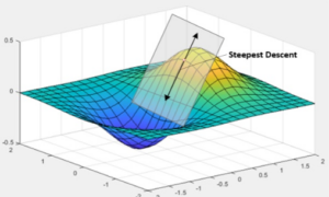
 Figure 1.4: Steepest Descent
If we walk down the hill toward the valley, we can define a plane that is tangential to any point at any moment, and in that exact point there is only one direction when the function would have the smallest loss, meaning the gradient is the steepest.
General approach to calculating the gradient descent can be represented like this:


So that is just about enough of theory, now we should understand how deep learning neural networks work at least at a conceptual level.
Let us now go ahead and start with a simple project, so that we can understand how all different pieces work together. You will need this:
- R Studio with R
- Anaconda (if on Windows)
- TensorFlow
- Keras
Let us install all these so that we can have our environment ready.
Installing RStudio and R
R is a programming language created for science, with thousands of libraries for almost any work you can imagine. We are here interested in machine learning packages, but first we need to install the RStudio. So, go ahead to this location and install the latest version of R first (version 4.0 was the latest one at the time of this post):
Then go here and install the free version of RStudio:
Open RStudio, you should see something like this:
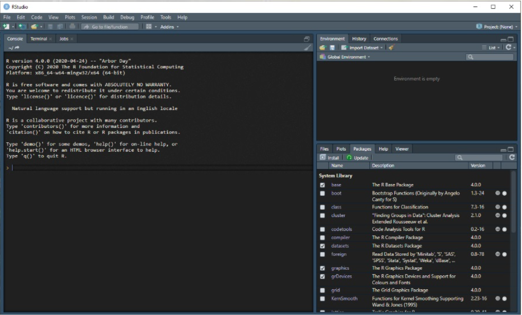
Figure 1.5: RStudio
As you can see, it displays the R version 4.0.0 in the console. Quick orientation here: in the console you type the commands, but you can also go File -> New File -> R Script, and type in the script, save it, then execute the script. Top right window will show the environment objects and their values, and to the bottom right side you have packages or files. You can install the packages from here, but it is more common you would do that from the Console itself. This is just an absolute minimum, there are of course many more features to RStudio, but this should get you started.
Install Anaconda
Install Anaconda Individual from this location:
It is a toolkit for using Python or R for your data science projects, and you need it if installing TensorFlow through RStudio, as we shall be doing. You can also decide to skip this step, and then you shall be asked to install Miniconda during the TensorFlow installation in RStudio, since TensorFlow is distributed as python packages so there needs to be a python environment installed on your box.
Install TensorFlow 2.0
Open RStudio, and type the following in the console:


If you have not installed Anaconda in the previous step, you will be asked to install Miniconda at this point. Accept it, and then just lean back and wait while all the packages are installed. It can take up to a minute, depending on your network connection.
Now execute the following two lines in the RStudio console:

This will select the tensorflow library (go to the bottom right window and you can see that this package has been selected), and then the second command install the tensorflow. Now if you type the following two command:
…you can assert that the TensorFlow is installed properly (see the third in white color, as above).
It is important to note several things here…first, it is recommended to use UNIX like systems for RStudio, TensorFlow and Keras. Secondly, if you are doing a true demanding data science work, then you need a great graphic card, in order to run these computations on GPU, rather than on CPU.
You can look for Nvidia CUDA enabled graphic cards here: https://developer.nvidia.com/cuda-gpus
CUDA is a toolkit created by Nvidia that increases the computational performance of linear algebra, deep learning, images processing and many other domains, which makes it perfect when running demanding computational training of neural networks. Of course, for a real work you should go for something like Nvidia Titan RTX which is based on Turing architecture, and uses the Tensor Cores to immensely improve the artificial intelligence computational speed, but cards like this usually go around $2,500 or so, so it is a pretty pricy toy.
The other choice would be to run the computations on Google cloud or Microsoft Azure. For instance, in Microsoft Azure you can shoot for machine learning processing on dedicated machine which use Nvidia Tesla cards, but this option also does not get cheat if you are doing serious work with deep learning networks and images processing for instance, or such.
When I say UNIX based system, that basically means either Mac or some Linux distro. Again, Mac is a worst choice, since those machines usually do not use Nvidia graphic cards, which leaves you with the Linux then. You should use either Ubuntu, or some distro that was forked out of Ubuntu, like Linux Mint or such. Those work best in my personal experience.
In any case, please bear in mind that you can install all these running on CPU, which would suffice for playing and testing, as in this post, but the processing of even medium-size deep neural networks is likely to take 3-5 hours on CPU, rather than less than 30 minutes if ran on GPU with CUDA.
Keras
Same as TensorFlow, we execute the following command in RStudio console:


Before this, you should create a new R session since it may complain about some dlls being in use or something. Then you go:


This will install the CPU version of Keras. If you have Nvidia graphic card as noted above in the previous section, then you should use this command instead:


Checking the current version is also easy, for instance:


Now this completes the setup of the environment, we now should have RStudio installed, R, TensorFlow and Keras library.
Let us now briefly make an introduction on what the TensorFlow and Keras are, and then we would go on creating the test project to put everything together.
This library is using data flow graphs with nodes that represent various mathematical computations, while the borders of these graphs represent the tensors, or multidimensional arrays. Since our interest is primarily in interfacing from RStudio to TensorFlow, it would be out of the scope to go into the internals of the TensorFlow itself, but it is worth noting that the notion of using data flow graphs provides for maximum parallelism when running the operations, it is easy to distribute the execution over multiple different machines, data flow graph is language independent so it has a high degree of portability, etc. When we write the code in R using Keras library that uses TensorFlow as backend engine, it automatically creates the TensorFlow graphs in the background, so it is transparent for us. In effect we use R language as an interface to TensorFlow.
The internal architecture of TensorFlow is very complicated, but if you are interested you can find more information here: https://www.tensorflow.org/tfx/serving/architecture
Keras is a deep learning framework, that makes it easier to use neural networks for machine learning. It is important to note that it is distributed under permissive MIT license, meaning it can be freely used even in commercial products.
Keras makes it much easier to create and use neural networks at a high level, but uses the TensorFlow as its backed to manipulate the tensors at a low level. It is not the only backend engine it can use, you can for instance use the Microsoft Cognitive Toolkit as well, with probably even more engines as well.
Without going into too much theory about this, let us start with an example projects, and it will become clearer on how this library is used.
We are going to use the Adult dataset from the UCI Machine Learning datasets, that shows census data about various persons in a multivariate data set. Our task is to create and train a model that predicts if the income will exceed $50K or not.
The process of a typical machine learning experiment goes like this:
- We get data, from somewhere.
- We normalize data, remove missing values, and do any other needed cleaning up.
- We the split the data into a train set and test set (usually 80%/20%, or something).
- We then create a neural network and set its layers and other properties.
- We then train the model using this network on the train data set.
- After the model has been trained, we then use the test data and gather the output on what the model would predict.
- We then compare the predictions with the real values in the train set, to determine the accuracy.
Of course, there is a lot more going on in here, but it is nice to understand the general flow of the prediction experiment.
Back to RStudio, we are going to create a script and then go step by step and explain what we are doing. If we look at the repository location, we can see general data about the set we will be working for:
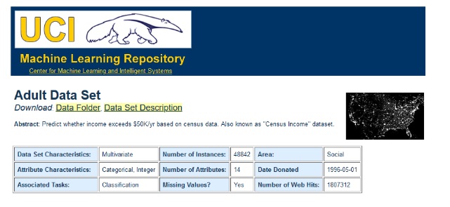

It contains adult census data, and the task is to try to predict the income value, as we shall se later in the text. The way we do it here is like a walk in the park, but the reality is never this beautiful. You would spend many days or even weeks processing data, gathering it from various sources and different formats, and doing lots of transformations to get something meaningful. Then you would go through data and try to normalize it and make it as convenient for the machine learning as possible. For instance, the native_country filed would likely be capacitated into the continents, to have a fewer of them, rather than many different states which increases the analysis and can even lead to overfitting. This is a common task and is performed after the data is loaded but before it has been split into training and test sets and prepared for processing. In our example we are just using a dataset that is ready, so it works quite nice for us.
Please go to File -> New File -> R Script and add a new script with some name of your choosing, then type this:

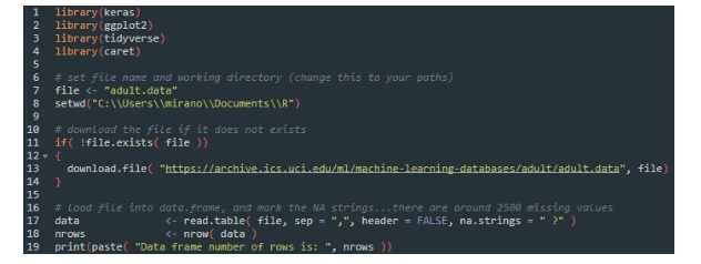
In line 13 we go and fetch the adult.data file from the url location, and save it in the local folder (second argument of the download.file command). We then go and create a R data.frame by loading the local file with read.table command. After that, we fetch the number of rows, and display it.
Now run this script…. either click Ctrl+Shift+S or go to the top right toolbar in the Script windows and click on Source to run the script.
Let us now see what is inside the data object, please execute head(data,10) command in the console window:


Executing command head(data, 10) displays the first 10 observations (or rows) from the data frame. Since we do not have columns, we can see that the data frame has automatically assigned values V1 to V15 to it. First 14 attributes (or columns) contain data and the last attribute (or column) is also called a label, since it contains the value that needs to be predicted. It would be better if we now add the column names to the data, so let’s add the following lines and execute the script again:


If we now execute the same command again: head(data,10), we shall see that the column names appear:


Let us now go to the top right window in RStudio named Environment, and click on the icon as shown below, in order to display the content of the data frame named data:

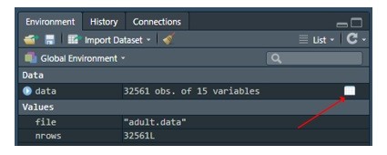
If you now scroll down a few times through this data frame, you should see the workclass and occupation and some other variables having a value NA, meaning they do not exist. We marked them this way when we loaded the data frame. Interesting fact is that the command read.table actually returns the object called tibble, and read.csv returns a regular R data frame. Tibble is more modern, lazy loads and forces you to do more work since it does not do stuff for you that data frame does.
Let us now get rid of these observations that have missing values, as it can make our training inaccurate. We do this by executing command as shown in lines 26-29 below:


If we execute the whole script now, we can see that we have removed around 2500 observations from the set:


Before we go any further, it would be good to remind us that our task is to train the neural network to make as precise prediction as possible on the label. We do that by splitting this dataset into 2 datasets: one contains 80% of the data, that we will be using to train the neural network, and the rest 20% that we will use to test the created model on how well it predicts the value for the label.
This is essentially a machine learning using supervised method, where we try to predict if the label will be either <=50K or >50K, meaning it is a classification task.
Let us quickly see the shape of the data when it comes to the label variable. We can display it in a histogram, but we first need to install the package ggplot (do not use script, run and execute this in the console window):


This will plot a histogram which shows the age of the person on the Y axes, and the income on the Y axes, showing an uneven distribution of the income where there are much more incomes that are below $50K (something like 75% of the incomes below $50K to 25% of income that are above $50K):

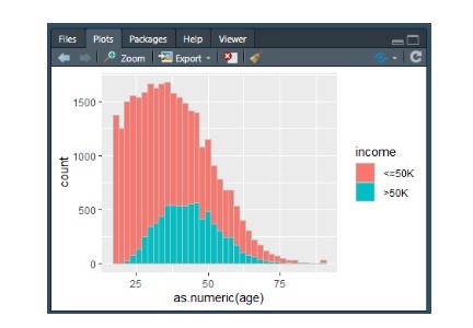
Looking the shape of data from many angles is what you would be doing a lot in this phase, to understand what the data represents and how various variable correlate to each other.
The next step is to do something called one-hot encoding….this is an important step, and usually is the one that takes some effort. The reason is that we cannot just feed the neural network with some data object that has a number of text columns, as machine learning is not working with texts but with numbers….and usually numbers normalized between 0 and 1.
Keep in mind the data set you have seen it in the previous steps, so bunch of data that has 15 columns (variables) and over 30000 rows (observations). Now let us add these commands as shown below in lines 32-41 to the script, and then execute the whole script again:


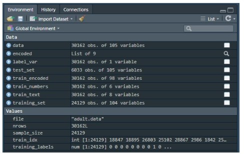
In the lines 32 and 33 we are creating new data frames that will receive data from the main data object. Depending whether the data type is a character or a number, so to separate them….the train_text will end up with 8 variables, and train_numbers will end up with 6 variables (so total of 14). You can go to the top right window named Environment and look it up by clicking on the table-like icon, as we have done it before, so that you can visually see what’s in there. Remember, we have selected this out of the first 14 variables, there is still one left which is the right-most variable, that is our label.
We then encode the train_text in lines 36 and 37, creating a new data frame named train_encoded. Now if you have visualized the train_text data, you can see that each of the columns would have a number of different values, which usually repeats, so there is a finite number of different values for each column. What we want to do is to encode these values and transform them into numbers, and then select the appropriate value in that column. Since we have done that already, you can now visualize the train_encoded data…this set has 98 variables, because each unique value from each variable was added to a new column, and then the appropriate column was added the value 1. Scroll horizontally the train_encoded and you would see the column names and how it is distributed.
We then go and extract the last variable, column 15th, into label_var, and then we bind all three data objects together into the original data object. Visualize the data object now, please note that it now has 105 variables: 98 one-hot encoded text variables, plus 6 variables that were already numbers, and then 1 additional variable which is our label variable. If you visualize it, you may need to click the paging button on the filter toolbar, as it will present the data in pages, then scroll to the right.
Cool…now let us split the data frame into two sets, one 80% and the other 20% of the observations…please add these commands to the script, and then execute the whole script again:


We create the index and then split the data into two sets: training_set that will contain 24129 observations of 105 variables (this is 80%), and test_set that contains 6033 observations of 105 variables (so 20%).
Now we need to transform the labels from both the training and test sets, and convert them to a number representation…please add lines 53-55 below, and then execute the script:


In line 53 we convert the label column data into numeric list, and since it will transform the original values of “>50K” and “<=50K” into 1 and 2, we then subtract 1 from the whole array to get 0 and 1…then we remove the column income, i.e. our label, from the training set. If you check the Environment window, you should see something like this now (note the training_labels values):
We then need to do the same on the test_set:

This concludes the data preparation phase, we now go and create the model, compile it, and add it to the fit function to start the model training:


In lines 63 and 64 we convert out data frames into matrix, as this is the type of data these layers expect, and then in lines 67 to 73 we create the sequential stack of layers from Keras, where we would have 2 layers and one output layer (see figure 1.1 above in the previous text).
We use the RELU or Rectified Linear Activation Unit for activation of the layers. The reason is that for this kind of classification challenges it is better suited than using nonlinear activation functions, such as sigmoid or hyperbolic tangent (TANH), as they saturate easily when they approach large or small values, and are only sensitive to changes around the middle. The TANH is just the relationship between the hyperbolic cosine and hyperbolic cosine, so it looks like this:


On the other side, the rectified linear activation unit plays nicely if we use the Stochastic Gradient Descent function for optimizer as it acts linear but is really not and thus allows for complex relationships to be learned in the backpropagation of the deep learning network. Since the classification model we are building is a binary problem, we need one output neuron, hence the sigmoid activation which provides us with just that.
Dropouts are used to drop the connections between the layers using the probability, for the purpose of regularizing the model.
Now the model is created, let us compile it:


In the compile step, we set the loss function, the optimizer, and the metrics. Now we add all these to the fit function, that starts the training:

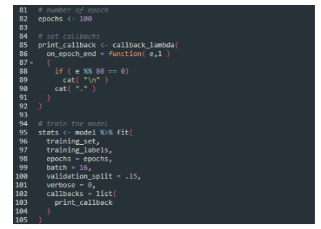
In the line 82 above we set the number of epochs to 100…the epoch is one full training cycle on the training set. After that, we call the model fit function and pass the parameters. Please note the callback function that is inserted as a parameter as well.
If you run the script now, it will start and you will see the results per each epoch in the console window, like this:
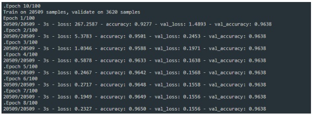
Also, in the Viewer window in the bottom-right part of RStudio, you would see an interactive progress, something like this:

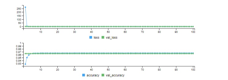
After a few minutes, the training will complete. We can then run the command plot(stats) in the console window, which gives us this diagram:

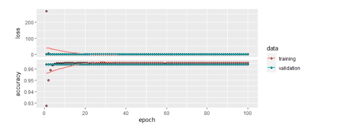
We can easily see in both diagrams that the loss function is very high in the beginning, and the accuracy is lower when the training starts (this is because weights are added randomly at the beginning of the training), and then quickly improves but than it does not change almost until the end. The accuracy starts from around 0.9366 (so 93.6% of accuracy)in first epochand goes up to 0.9653 in about 10 epochs only.This means that we can further improve the process by specifying that if for some n number of epochs the accuracy does not improve more than x value, then the training can stop, so to avoid the overfitting the model.
Let us do this…add the early stopping callback, as in lines 94-95 below, and then add it to the callback list of the fit function parameters (line 107):

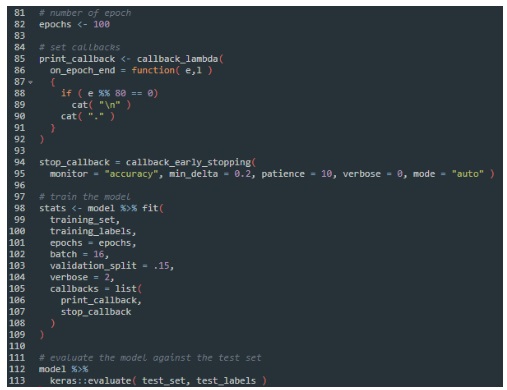
We also add the evaluate function, as in lines 112-113 above, to evaluate the test set using the trained model.
After we run the script this time, we can see that the number of epoch ran is around 12 now, since the accuracy does not improve for more than 0.2 in 10 epochs (as we set in the callback function), the training stops:

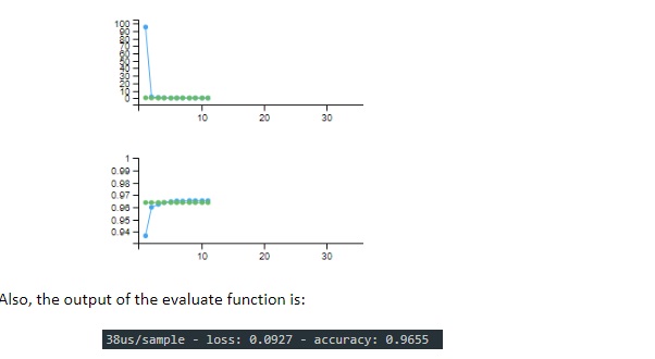
So pretty good, we have achieved the 96.5% accuracy without doing too much work or tweaking different activation functions or directly dealing with weights and biases to improve the result even more.
Using Keras in RStudio with TensorFlow backend provides a very convenient way for creating neural networks. There are many convenient functionality to this, such as the ability to run under CPU and GPU without any changes to the code, the API is pretty user-friendly and can be easily understood, it provides for creating many different neural networks, with an easy configuration, can use TensorFlow as backend engine but also other engines can be plugged in.
BIBLIOGRAPHY
Atienza, Rowel. “Advanced Deep Learning with TensorFlow 2 and Keras”. Packt Publishing. ISBN 9781838821654.
Chollet, Francois. “Deep Learning with R”. Manning Publications, Meap Version 1.
Dean, Jeff; Monga, Rajat. “TensorFlow:Large-Scale Machine Learning on Heterogeneous Systems”. TensorFlor.org. Retrieved May 3rd, 2020.
Falbel, Daniel; Allaire, JJ; Chollet, Francois. “Keras R Interface”. CRAN. Retrieved May 3rd, 2020.
Galeone, Paolo. “Hands-On Neural Networks with TensorFlow 2.0”. Packt Publishing. ISBN 9781789615555.
“Machine Learning Crash Course with TensorFlow API”. Google.com. Retrieved May 3rd, 2020.
Moocarme, Matthew. “Applied Deep Learning with Keras”. Packt Publishing. ISBN 9781789950922.
Pawlus, Michael; Devine, Rodger. “Hands-On Deep Learning with R”, Packt Publishing, ISBN 978-1-78899-683-9.
“R Interface to TensorFlow”. TensorFlow Authors and RStudio. Retrieved May 3rd, 2020.
Shukla, Nishant. “Machine Learning with TensorFlow”. Manning Publications, ISBN: 9781617293870. Verzani, John. “Getting Started with RStudio”. O’Reilly Media, ISBN 9781449309039.


