Intro to Face Recognition in R
Humans are very quick to detect and recognize faces, and the entire process executes in a matter of fractions of a second. Doing the same with a computer proves to be much more challenging.
There have been many solutions proposed in the past 50 or more years, but none of the solution seems to be a clear best one, even though they do work in practice and yield some spectacular results. The most appealing reason for using face recognition for identification is that it is non-invasive, meaning you do not need a subject to cooperate as is the case with fingerprint analysis or retina scan. We can use facial recognition for protecting our privacy or our assets in places where we today use PINs for ATM transactions or type in various passwords. Unfortunately, it can also be used for identification for other sinister reasons, that are beyond the scope of this article.
It is still unknown what cognitive processes are included in recognizing faces and how it all works, but there are many other inputs that are used, not just a visual one. For instance, the context plays role and the brain uses it to aid in facial recognition, to determine the face and the place in the context that face should belong to. It also seems that there is a separate system in the brain that governs most of the face recognition process, and that conclusion is drawn from the fact that faces are more easily remembers than other objects, so there must be some dedicated system for that. Also, patients who have prosopagnosia (https://en.wikipedia.org/wiki/Prosopagnosia), which is also called “face blindness”, in which they cannot recognize familiar faces but are still able to make difference between other objects or higher intellectual reasoning, leads to a conclusion that there is a system dedicated to face recognition only. People with prosopagnosia can find a nose, mouth and other details on the face, but are unable to put it all together in one face structure, so it must mean that the face recognition is more than merely visualizing face characteristics. (Zhao W. et al, 2003. Face recognition: A literature survey. Volume 35 Issue 4:399-458
Mathematical Approach
The mathematics behind the face recognition can be quite complex, but it would be interesting to at least touch upon the bare basics of it and present a few commonly used algorithms. If you are not interested in the underlying math at all, please skip to section 3. Microsoft Cognitive Services.
These are some of the frequently used approaches in face recognition, however as stated earlier none of them is a clear winner so we are yet to come up with the “perfect” algorithm for face recognition.
Principal Component Analysis (PCA):
The first approach in face recognition was made by Kirby and Sirovich in 1990 (Kirby, M. and Sirovich, L., 1990. Application of the Karhunen-Loeve Procedure for the Characterization of Human Faces. IEEE Transactions on Pattern Analysis and Machine Intelligence, vol. 12, no. 1).
This proposal is commonly called eigenfaces and is based on Principal Component Analysis, and has been improved and extended over the years to a number of similar solutions making it the most common face recognition algorithm today. It is based on reducing the dimensions by estimating a linear subspace that spans the samples. These orthogonal subspaces are actually eigenvectors of the image data covariance matrix, which are a special kind of vectors used in linear system of equations. They are usually used in industry and physics in general for calculating stability, vibrations of bodies, rotation, signal processing, machine learning etc.
There are left and right eigenvectors, where right ones are most commonly used. Having the square matrix A if we want to decompose it into eigenvector we apply eigenvector decomposition, so we can define the right eigenvector as a column XR vector that has

where A is a matrix, as mentioned above, so

yielding a conclusion that right eigenvectors have zero determinant:

So what we are trying to do using eigenvectors when tackling the problem of face recognition is to try to represent the image in terms of linear combination of eigenfaces, where we only used the eigenfaces with largest values, discarding the ones with lower values. This means that if we have a set of images in the process of face recognition A={ai:i=1..n}, and where each of the images in set has dimension p, we can solve it by using the following equation
 where a holds a p*n matrix of the normalized image vectors, and a with dash is the mean image of the face.
Linear Discriminant Analysis (LDA):
This approach is very different than Principal Component Analysis, and is based on calculating vectors that best discriminate among classes, as described in Belhumeur, Peter N. et al, 1997. Eigenfaces vs Fisherfaces: Recognition Using Class Specific Linear Projection, 713-714.
It is interesting that this algorithm tries to approach the face recognition problem from the perspective of minimizing the effects of light direction on the picture or various facial expressions by taking a pattern classification approach.
This analysis is based on computing the within-class and between-class scatter matrix, focusing on computing the directions that will represent the axis that maximize separation between multiple classes.
We can calculate the within-class scatter matrix using the following equation

where mi is the mean factor

The between-classes scatter matrix Sb can be calculated using
![]()
where mi is the overall mean, and mi and Ni are the sample mean and sizes of the classes.
An interesting point in using the LDA approach is detection of glasses, something which will be demonstrated later in part 3 where we will use Microsoft Cognitive Services to uncover if the person on image has glasses or not.
Using Gabor Wavelet (GW)
Wavelets are relatively new approach to the domain focusing on providing an optimal resolution in spatial and frequency domain, and it comprises of decomposing an image in sub-bands that are scaled and oriented in various ways. It is based on the Gaussian kernel which is modulated by sinusoidal wave (Tai, S. L., 1996. Image Representation Using 2D Gabor wavelets. IEEE Transactions on Pattern Analysis and Machine Intelligence , 18(10), 959–971).
This approach originates from the signal detection math, so the usage in face recognition is based on using the scalable window that moves over the image and we calculate the spectrum for every position, repeating this many times with modified windows in order to get a large collection of wavelet representations of the image.
Gabor wavelets can be expressed with the following equation:

where Z=I (x,y), and ∥.∥ is the normal operator, v = scale, u=orientation, v=wave vector and σ=Gaussian Window.
The application is usually based on rectangular shapes that are used to create the non-overlapping regions, and the touch points between those regions are where the image is decomposed into a set of wavelets, that has a different position and frequency as mentioned earlier. The process usually goes by passing the image through a number of filter stages where filter outputs are sampled in a horizontal direction.
Hidden Markov Models (HMM)
This approach is related to Hidden Markov Models, which is a robust mechanism that models each state separately for each facial region, as shows in figure 1.1. below. Each state represents a multivariate Gaussian distribution as probability density function. The idea is that we can scan the face top-down as it is common that the human head has forehead, eyes, nose, mouth and then a chin going from top to down.
Figure 1.1: Hidden Markov Models for Face Recognition
So the approach is to train the HMM on a huge database of images reading them all from top to bottom with each row read as feature vectors. Then we read it using the multivariate Gaussian distribution to model the distribution of vectors for that facial region, which is represented as an actual state.
We then use this approach to model each state S of the face to represent a distinct facial region, and inside each state S we use the probability density function within each state.
We are using the probability density functions (PDF) P(x) of a continuous distribution is defined as the derivative of the distributions function D(x):

which means that we have

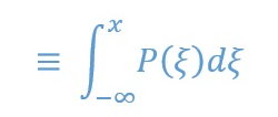
This implementations is actually one-dimensional, and it is used to iterate through all rows of the image, as shown below in figure 1.2:
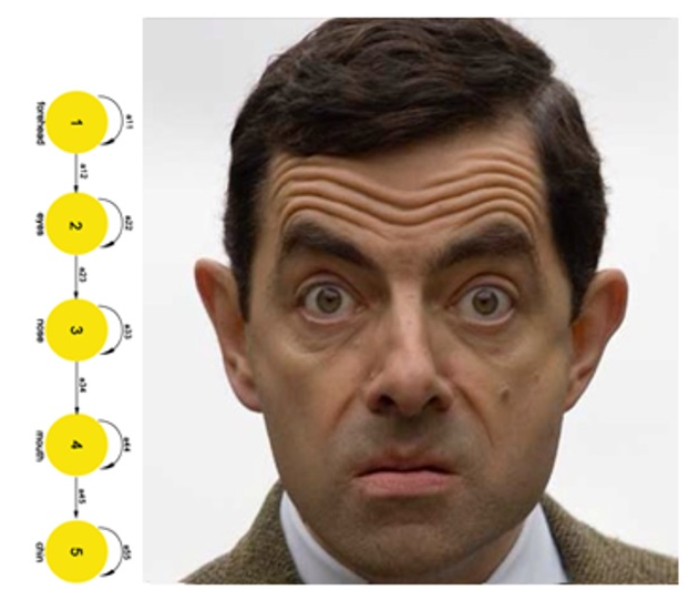
Figure 1.2: Hidden Markov Models for all five states
However, for this special challenge of face recognition, a slightly different implementation of the probability density function was used that is called a Gaussian Mixture Model, and it has been used within each state S we need to iterate through. The Gaussian Mixture Model is a continuous probabilistic representation widely used to estimate the uncertainty in the world. When it comes to one-dimensional Gaussian, it all boils down to interpreting the distributions that are otherwise easy to calculate, such as mean and variance. This is the normal or Gaussian distribution, which can be represented as:

The Central Limit Theory also stipulates that it is expected that mean of any random variable will converge to Gaussian. However, there are many cases where single Gaussian cannot fit the model, so we need to use the Gaussian Mixture Model, as is the case here in Hidden Markov Models. GMM has a mixture of component weights and component means and variances.
Let’s say we have a Gaussian mixture model with K components, the kth component has a mean of mK and variance of bK then the mixture component weights are defined as FiK for component cK having the constraint that Eki = 1 and Fi=1 in order to have the probability distribution to be normalized to 1, then:
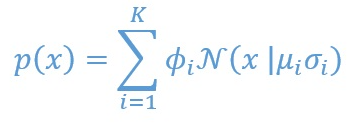
This is only a simple implementation of it, we then extrapolate the current top-down vertical model to also use the Hidden Markov Models for each of its states (vertical indices). This was elaborated in details by Radford M. Neal et al., 2003. Inferring State Sequences for Non-linear Systems with Embedded Hidden Markov Models, 2-4.
Microsoft Cognitive Services
Let’s now see how all this works in practice, by using Microsoft Cognitive Services. Microsoft Cognitive Services is essentially a set of APIs that offer various algorithms like vision, speech, language and others. You can find it at this location: https://azure.microsoft.com/en-us/services/cognitive-services/
First you would need to create an account or use an existing one to get the access. If you have an active Azure subscription, you can also enable it there. In any case, you would get 30.000 transactions per month, and up to 20 transactions per minute, which is sufficient for playing with this API and testing its capabilities.
We need not to cogitate over every aspect of cognitive services, better to dive right in. So what we want to do is to get an image and send it for detection with Face API, and then get the results back. Such results include detection of face points like general dimensions, pupil positions, nose tip and many others, but also include results calculated by machine learning algorithms which can show various face features, such as age, gender, pose, smile and many other.
In this exercise we would mainly focus on detecting the age and if the person at picture is showing some emotions and what those are, which would be sufficient to demonstrate the usage of this API.
So after you have subscribed to the API, please look for the keys as you would not be able to make calls against the API without them. If you have created a free account at Cognitive Services web page, then click on the Account link at the top right and you will see something like this:
 Figure 3.1: Cognitive Services Keys
If you prefer to use the Azure, then search for Cognitive Services and after create one you would be able to find your keys under Resource Management -> Keys. You can use either of two keys given to you.
It is now time to fire up the “R-Studio”. I would assume you were a beginner and never used R before, so would lead you step by step. If you already used R, then you can skip this paragraph.
Installing R and R Studio:
First install R itself by going to https://cran.rstudio.com/ and choosing the installer depending on your operating system. The installation is fairly straight-forward, just click Next every time in the installation dialog.
After that, we need to install the R-Studio by going to this location: https://www.rstudio.com/products/rstudio/download2/ . Choose RStudio Desktop free version, and from links below choose the appropriate installation based on your operating system:

Figure 3.2: RStudio Installation
After installing the RStudio, please run it and you would get the main application view:
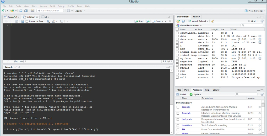
Figure 3.3: RStudio
I cannot go into details here, as this is not an introduction to RStudio, but it is important to note that there are 4 main areas that this applications displays:
- Top left you would find an area where the R script (or other types of scripts) are composed,
- Bottom left is the console, where you can type in the commands directly or see the results after the script has run,
- Top right is the list of variables and objects currently in your workspace, and
- Bottom right is various windows, like packages, plots, help and others.
Starting with RStudio:
I am on Windows, so I will give you the instructions for that OS, but other installations should be pretty much the same. We now need to connect to Face API and send a picture for detection. After you have fired up the RStudio, let’s go to toolbar and add a new R Script (this toolbar is the left-most one):

Figure 3.4: RStudio script
Now click Save toolbar or CTRL-S and RStudio will prompt you to save the file, give it some name (for instance, “TestFaceAPI”) and save it. Please note that the file is saved in your Documents folder as this is your root by default, but you can change it.
Go to console below and type getwd(), you will get something like this:

Figure 3.5: Executing command in console
This means your root is your default Documents folder. If you wish you can changed it by using setwd(“Some Other Folder”).
Now go to bottom right portion of your RStudio and click on packages, then click on Install right below it, and install the httr package by typing its name in Packages text box and clicking on Install. This package adds libraries that R needs to work over http.
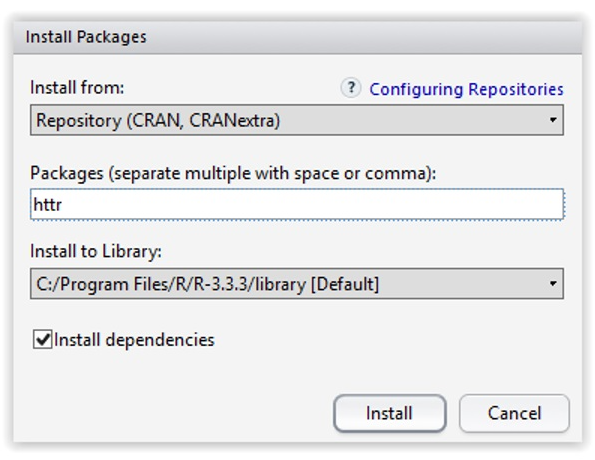
Figure 3.6: Installing the package
RStudio will do everything rest, after that you just need to go to packages again and check the httr package:
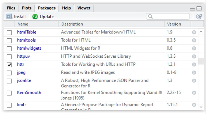
Figure 3.7: Selecting the package
You will notice this action makes RStudio to execute the command in the console window to the left.
Now let’s get back to our scrip above and ad the first line of the script:
baseUrl <- “https://eastus2.api.cognitive.microsoft.com/face/v1.0/detect” q <- “?returnFaceId=true&returnFaceLandmarks=true&returnFaceAttributes=age,gender,smile,headPosefacialHair,glasses,emotion” url <- paste(url, q, sep=””) |
Nothing fancy here, we are specifying the baseUrl variable, then query variable and concatenating that into the full url. Please note that the operator <- is the same as = operator, so assigns the value on the right to the variable defined on the left. As you can see, we want to get the dimensions and other landmarks of the face, along with the attributes like age, gender, smile and other. You can also add other values to face attributes parameter, like HeadPose, Glasses etc. Please consult the API documentation for the full list at this location:
Now on to finding the image for testing. We can use a local image stored on our computer, but for this exercise we would use the one in the image repository. One such nice repository can be found at the University of Massachussetts: http://vis-www.cs.umass.edu/lfw/
You can explore or download images, and you can also use any picture of course, but for the purpose of this blog I will use the Jack Nicholson’s pictures that can be found at this location: http://vis-www.cs.umass.edu/lfw/person/Jack_Nicholson.html
Let’s use the pictures in the left most column, second and third image from the top:
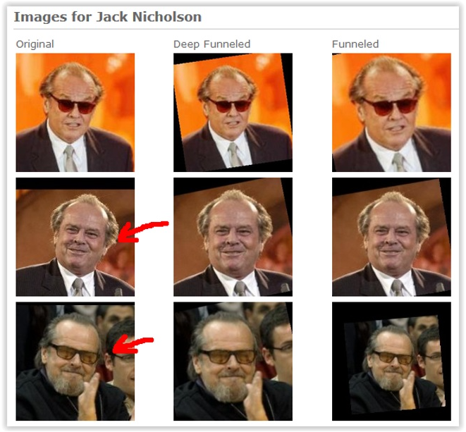
Figure 3.8: Pictures for testing
Let us now add the urls of these pictures to our R script, by adding these lines:
img1 <- “http://vis-www.cs.umass.edu/lfw/images/Jack_Nicholson/Jack_Nicholson_0002.jpg” img2 <- “http://vis-www.cs.umass.edu/lfw/images/Jack_Nicholson/Jack_Nicholson_0003.jpg” |
You R script should now look like this:

Figure 3.9: R-script code
As you can see, both pictures belong to the same person, but they are rather different: one in which he smiles and the other one where he has glasses and beard. This makes it even more interesting for face recognition process.
Let us now continue….we need to download these pictures, save them to temporary files and then load them in the format that can be used for sending a request to Face API. We can achieve that with the following code:
f1 <- tempfile() download.file(img1Url, f1, mode=”wb”) pic1 <- upload_file(f1) f2<- tempfile() download.file(img2Url, f2, mode=”wb”) pic2 <- upload_file(f2) |
Your code should look like this:

Figure 3.10: R-script code
As you can see, in line 8 we create variable f1 that points to a temporary file in temp folder, in line 9 we download the picture and write it to the file, and then in line 10 we load the picture from disk to variable pic1. Then we do the same for the second picture in lines 12-14.
Next is to call the cognitive services API and send the picture for detection. We do that using this code:
response = POST(url=url1, body=pic1, add_headers(.headers = c(‘Content-Type’=’application/octet-stream’, ‘Ocp-Apim-Subscription-Key’=’xxxxxxxxxxxxxxxxxxxxxxxxxxxxx’))) result <- content(response) df <- as.data.frame(result) |
Your code now should look like this:

Figure 3.11: R-script code
In line 16 we are preparing the request and sending it to the url of the endpoint defined in line 1 above. As you can see, we are sending the key with the request, so please change the xxxxxxxxxxxxxxxxxxxx in my code with a valid subscription key. I have explained in the text above how you can get that key.
In line 19 we fetch the results and then convert the result to a standard R data frame structure. Data frame is probably the most important and heavily used structure in R, but it is sufficient to know that it is just like a table with rows and columns, and we need not to delve into that data structure to a great extent.
Now it is time to run the code and see what we get. Before that, let’s make sure we have all libraries loaded….since command upload_file in lines 10 and 14 requires us to use the jpeg package, let’s make sure it is loaded in the workspace by going to the packages in the lower right panel, and selecting it:
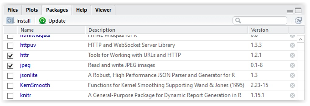
Figure 3.12: Selecting packages
The httr package was already selected earlier, as R needs it to execute the request over http.
If you have done everything correctly, then you need to save the script by clicking on the Save toolbar button or just CTRL-S, and then run the code with “Source” command that you can find here:

Figure 3.13: Sourcing the script file
The “source” command just reads the R code from a file and runs it in the console. You will see some lines executed in the console, and now you need to go to the “Environment” tab in the upper right panel, find the df data frame and to the right you will see a button that has an icon that looks like a table, please click on it:

Figure 3.14: Resulting data frame
After you click on the data frame, you will be able to see its content in the main panel right next to our R script:

Figure 3.15: Resulting data frame
As you can see, our data frame has one row and many columns in it. The column names are pretty self-descriptive…please scroll to the right and see what it contains. You can see that there are many measures of face and its borders, like rectangle in which the face is located in, then like positions of pupils, nose, mouth etc. If you scroll all the way the right you can find even more interesting data, such as:
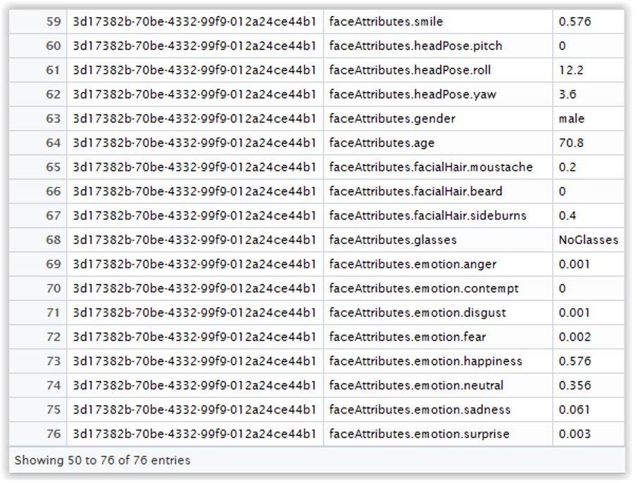
Figure 3.16: Resulting data frame
Don’t worry, I just pivoted the data frame in order to better see the data as rows rather than as the columns. You can achieve that with this command:
# pivot the data frame…you need to add package reshape2 for this df2 <- melt(df, id=c(“faceId”)) |
Now looking at figure 3.16. above we can find the smile property, which indicates that there is a 58% the person is smiling, then it has detected the person is male, age 70.8, no beard, no glasses….and also some other interesting emotions. All at all the results are pretty impressive I would say, and rather correct.
It is also interesting to note that these emotions like sadness, surprise or fear are chosen as they are recognized to be similar over different races and cultures, so they work in most of the cases.
Let us not play some more to see if the dimensions are correct as well. The RStudio has the plot area, as R is used in data science so it is only natural that it has very strong graphical capabilities.
I am not going to explain the plotting and drawing a raster image right now, as it can get complicated since there are many parameters to those functions. Let us just type the code like this:
img1 <- readJPEG(f1) plot(0:1, 0:1, xlim=range(c(0,150)), ylim=range(c(0,150)),type=’n’, asp=1) rasterImage(img1, 0, 0, 150, 150, interpolate=F) |
… so your script should now look like this:
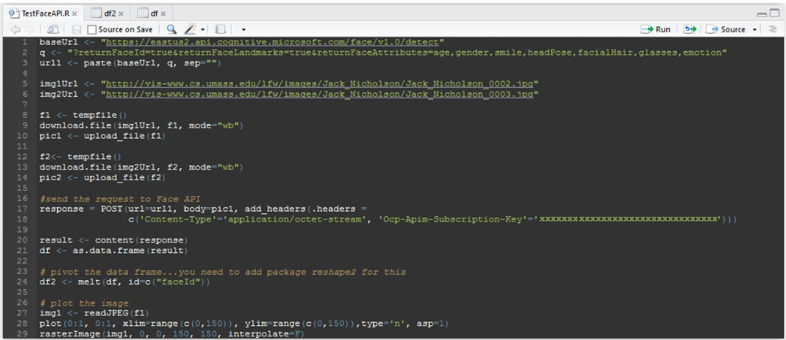
Figure 3.17: Plotting the image
So as you can see, in line 27 we are reading the image from file and plotting it in the coordinate system with parameters as show in line 28, then drawing the image in that area in its original dimensions. The aspect ratio is set to 1 so we do not distort the image. If you want to learn more about the plot or rasterImage functions and their parameters, please type ?plot or ?rasterImage in the console, and help file will open to the right with more information about these functions.
Now save the script and click on “Source” button again to execute it. After it has finished executing, go to the lower right panel, click on Plots tab and you should see something like this:
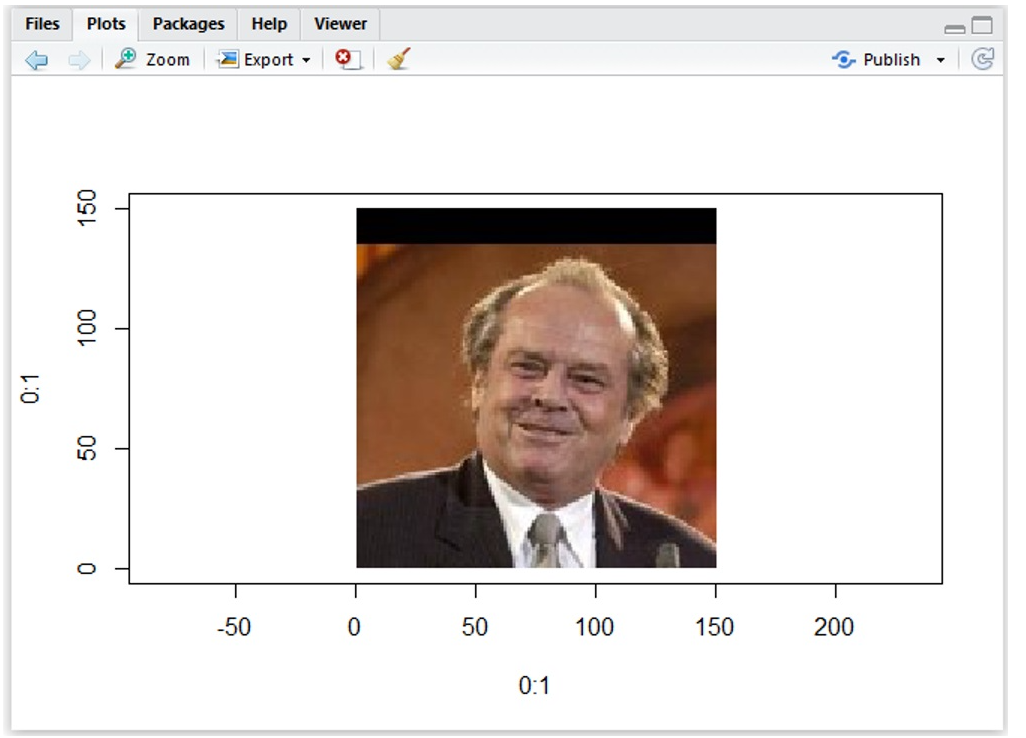
Figure 3.18: Image in the plot area
The picture was displayed in the coordinate system from x = 0 to y = 150, which is actually the height of the image that is a square. Let us now try to use the data we have received in the response from Face API, and try to find the tip of the nose, or the location of the pupil.
Since the picture is has already been drawn, we can now fetch the data from our data frame and just draw the dots on the image. Let’s add the following lines of code to the end of our R script:
# tip of the nose tip_nose_x = df[ ,c(“faceLandmarks.noseTip.x”)] tip_nose_y = df[ ,c(“faceLandmarks.noseTip.y”)] #now let’s draw the dot at that location points(tip_nose_x, tip_nose_y, pch=19, col=”red”) |
The full code should now look like this:
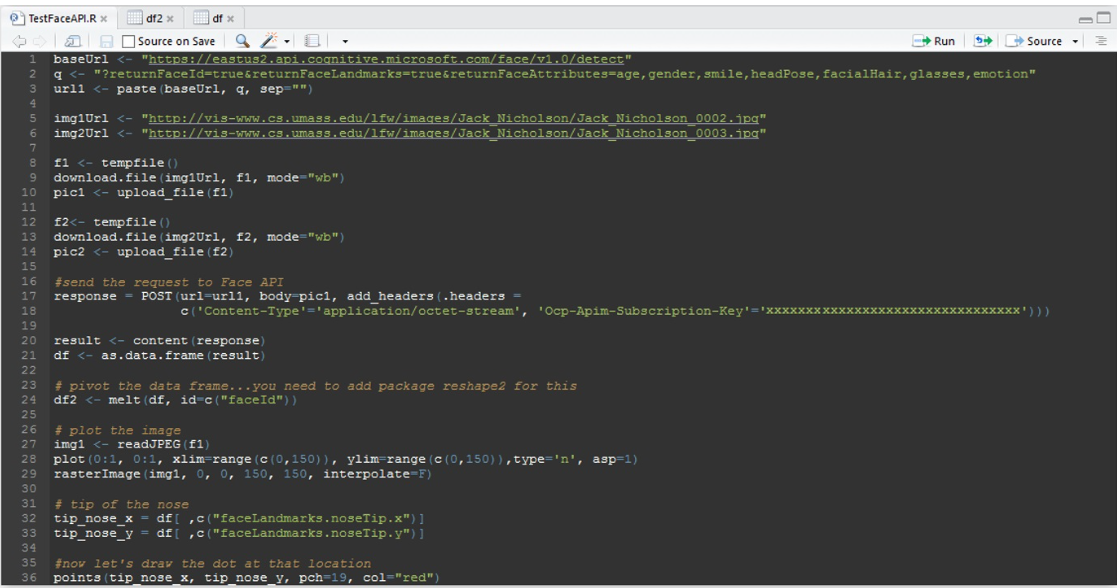
Figure 3.19: R script so far
As you can see, in line 32 and 33 we are extracting the values for nose tip, and then in line 36 we are drawing it over the image.
Now please execute the code with “Source” command and go the plot area…you will see something like this:
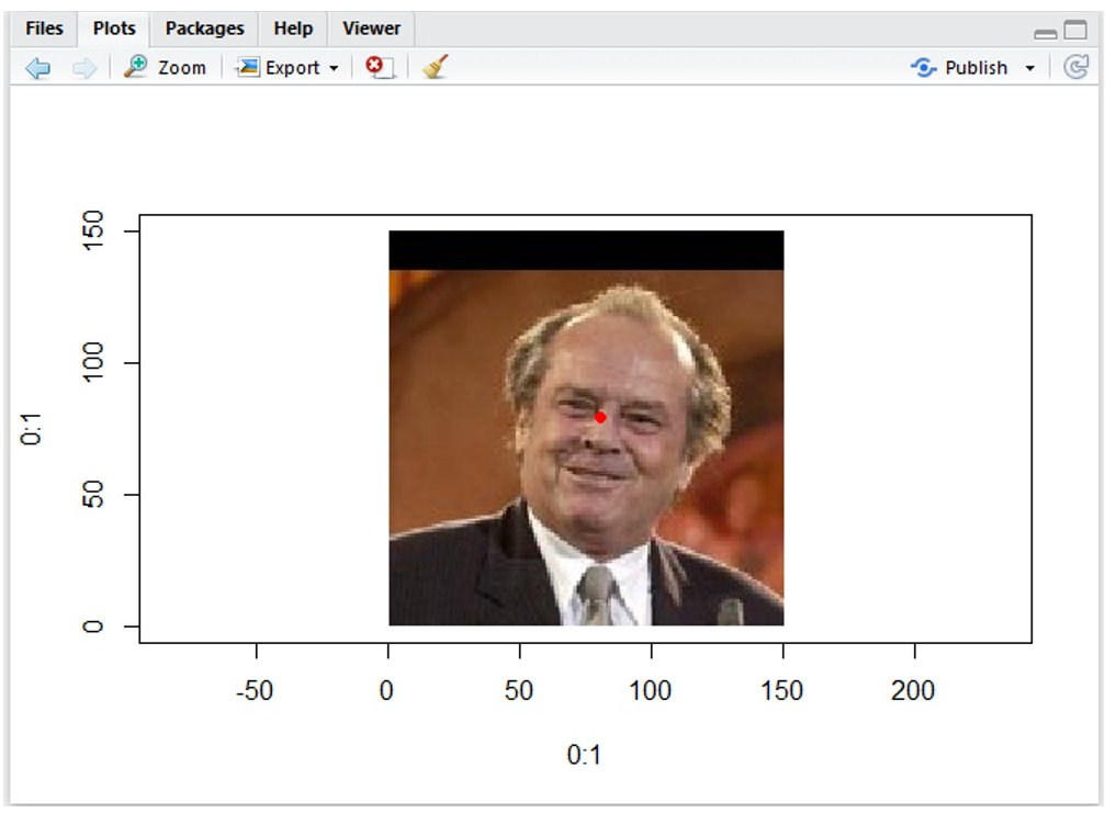
Figure 3.20: Drawing point at the tip of the nose
As you can see, the result is not really very precise. What is the problem? Well we have a coordinate system that is a classical Cartesian coordinate system, in which the coordinates are signed distances to the point from the two fixed perpendicular direct lines, and these lines are measures in the same units:
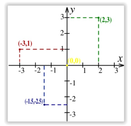
Figure 3.21: Cartesian coordinate system
So the coordinate 5,5 would be 5 units to the right and 5 units to the top from the x axis…however what we have extracted in our code was the x and y coordinate of the tip of the nose, which was exactly x=80.3 and y=70.6, however the y measurement does not point to the location on the y axis but rather the distance from the top of the image.
The solution is very simple, we just need to subtract the y coordinate from the image height, so let’s do that:
# tip of the nose tip_nose_x = df[ ,c(“faceLandmarks.noseTip.x”)] tip_nose_y = df[ ,c(“faceLandmarks.noseTip.y”)] IMAGE_HEIGHT <- 150 #now let’s draw the dot at that location points(tip_nose_x, IMAGE_HEIGHT – tip_nose_y, pch=19, col=”red”) |
Your code should now look like this:
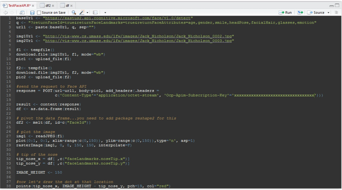
Figure 3.22: Corrected code for drawing dot on the tip of the nose
Now let’s execute the code with “Source” command, and open the plot area, it should resemble this figure:
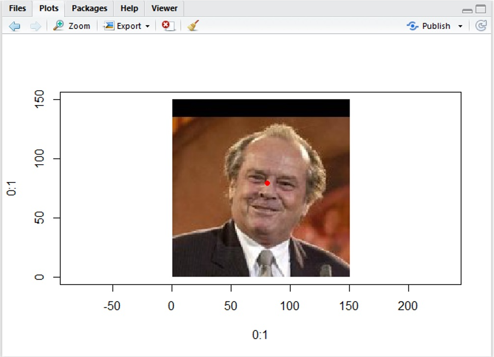
Figure 3.23: Drawing point at the tip of the nose – corrected
Looks much better, right? Let’s do the same but now for the left pupil:
#now let’s draw the dot at that location points(tip_nose_x, IMAGE_HEIGHT – tip_nose_y, pch=19, col=”red”) # left pupil location left_pupil_x = df[ ,c(“faceLandmarks.pupilLeft.x”)] left_pupil_y = df[ ,c(“faceLandmarks.pupilLeft.y”)] points(left_pupil_x, IMAGE_HEIGHT – left_pupil_y, pch=19, col=”red”) |
The complete code should lool like this:
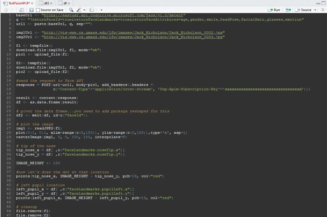
Figure 3.24: Code for showing the position of the left pupil
So we are essentially doing the same as before, getting the x and y position of the left pupil (or rather the right on, if not looking from our perspective), and displaying it on the image. Please also note the lines 46 and 47, we are cleaning up the temporary files we have created earlier.
Run the code now with “Source” and look at the plot:
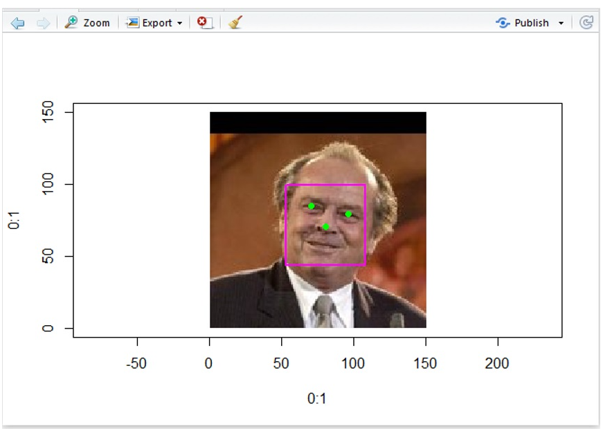
Figure 3.25: Showing the position of the left pupil
Let’s now add the code to show the other pupil, and also to draw the rectangle of the face. If you look more closely, you will notice that the resulting data frame df2 has three different variable groups: faceRectangle, faceLandmarks and faceAttributes. We use faceRectangle to draw this rectangle, so:
# right pupil location right_pupil_x = df[ ,c(“faceLandmarks.pupilRight.x”)] right_pupil_y = df[ ,c(“faceLandmarks.pupilRight.y”)] points(right_pupil_x, IMAGE_HEIGHT – right_pupil_y, pch=19, col=”green”) # face rectangle xleft <- df[ ,c(“faceRectangle.left”)] ytop <- IMAGE_HEIGHT – df[ ,c(“faceRectangle.top”)] ybottom <- ytop – df[ ,c(“faceRectangle.height”)] xright <- df[ ,c(“faceRectangle.left”)] + df[ ,c(“faceRectangle.width”)] rect(xleft, ybottom, xright, ytop, col=NA, border=”magenta”, lwd=2) |
If you run the code now, you should get the results similar to this:
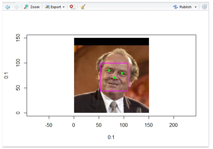
Figure 3.26: Race rectangle
I have also changed the color of dots showing the position of his pupils and the tip of his nose to green, just to get rid of that freakish red color coming out of the eyes.
You can continue playing with this yourself and trying to find the position of other landmarks returned by the service.
Now let us do the last exercise comparing two images as shown in figure 3.8 to determine what is the confidence level the person is the same on both pictures. As you can see, he has beard and glasses on the other picture so they are rather different at first sight.
The second picture was loaded earlier in lines 12-14 of out script, so we can now send it for processing the same way we did with the first picture:
#send the second picture to Face API response = POST(url=url1, body=pic2, add_headers(.headers = c(‘Content-Type’=’application/octet-stream’, ‘Ocp-Apim-Subscription-Key’=’xxxxxxxxxxxxxxxxxxxxxxxxxxxxx’))) result2 <- content(response) dfSecondPicture <- as.data.frame(result2) # pivot the data frame dfSecondPicturePivoted <- melt(dfSecondPicture, id=c(“faceId”)) |
Let’s select the data frame dfSecondPicturePivoted from the list of environment variables, and open it by clicking the table-like icon on the right, we would get something like this:
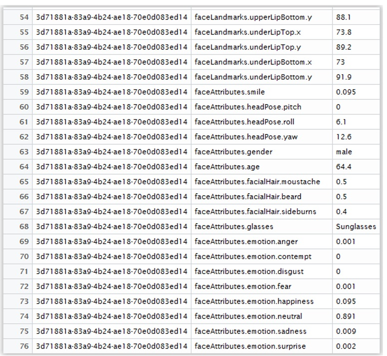
Figure 3.27: Results for second image
Examining rows 65, 66 and 68 we can see that it has detected beard and moustache with the confidence level of 50% (not a full bear, so it looks about right), and also that he is wearing sunglasses.
Now we would like to determine if two pictures belong to the same person, as Jack looks rather different on them. For that, we would need to get the unique id of the picture after it has been process by service with call using the detect endpoint. So here’s the code:
# detect similarity pic1FaceId <- df[,c(“faceId”)] pic2FaceId <- dfSecondPicture[ ,c(“faceId”)] baseUrlFindSimilar <- “https://eastus2.api.cognitive.microsoft.com/face/v1.0/findsimilars” bodyFindSimilar <- sprintf(‘{“faceId”: “%s”, “faceIds”: [“%s”, “%s”], “mode”: “%s”}’, pic1FaceId, pic1FaceId, pic2FaceId, “matchPerson”) #send pictures to Face API – Find Similar responseSimilar = POST(url=baseUrlFindSimilar, body=bodyFindSimilar, add_headers(.headers = c(‘Content-Type’=’application/json’, ‘Ocp-Apim-Subscription-Key’=’xxxxxxxxxxxxxxxxxxxxxxxxxxxxxxxxxxxx’))) resultSimilar <- content(responseSimilar) dfSimilar <- as.data.frame(resultSimilar) cat(“\n”, “Similarity between first picture and itself: “, dfSimilar[,c(“confidence”)]) cat(“\n”, “Similarity between first and second picture: “, dfSimilar[,c(“confidence.1”)]) |
The code should now look like this:
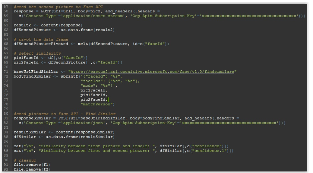
Figure 3.28: Detecting similarity between faces
So in lines 68-69 we fetch the ids of pictures we sent for processing at detect endpoint, as these are already processed and remain accessibly at service side for another 24 hours.
Line 71 is the base url of this API method, and lines 72-78 we create a JSON body payload, as this method requires all parameters to be passed in a body as application/json. We use faceIds parameter here, but it is also possible to use faceListId parameter and pass the previously created list on the service side, which remains persisted indefinitely.
After that in lines 81-85 we compose the request and send it, then process the response and convert it to data frame. Lines 87-88 just format and print the result in console.
If all went well, you can then find the dfSimilar data frame in the list of object in the Global Environment list, and clicking it you will see the following:

Figure 3.29: Result of detecting similarity between faces
We can see that the first picture similarity to itself is 1, meaning 100% (we used this as a control variable), and its similarity with second picture would be 0.55, so 55%, which seems okay to me.
If you survived to this point then maybe you can continue to play with other interested calculations you can get from the Face recognition API, and you may also try to use other APIs in the cognitive services, like speech, text etc. Enjoy!
Full code: https://github.com/mirano-galijasevic/DeepLearning/blob/master/AdultCensusClassifier.r
BIBLIOGRAPHY
Belhumeur, Peter N., Hespanha, Joao P., Kriegeman, David J., 1997. Eigenfaces vs Fisherfaces: Recognition Using Class Specific Linear Projection, 713-714, from https://cseweb.ucsd.edu/classes/wi14/cse152-a/fisherface-pami97.pdf.
Byun, B., Lee, C. H., Webb, S., & Pu, C., 2007. A Discriminative Classifier Learning Approach to Image Modeling and Spam Image Identification. Proceedings of 4th Conference on Email and Anti-Spam, (CEAS-2007).
Kirby, M. and Sirovich, L., 1990. Application of the Karhunen-Loeve Procedure for the Characterization of Human Faces. IEEE Transactions on Pattern Analysis and Machine Intelligence, vol. 12, no. 1
Meera, M., & Wilsey, M., 2015. Image Forgery Detection Based on Gabor Wavelets and Local Phase Quantization. Proceedings of Second International Symposium on Computer Vision and the Internet (VisionNet’15), 76-83
Radford M. Neal, Matthew J. Beal, and Sam T. Roweis, 2003. Inferring State Sequences for Non-linear Systems with Embedded Hidden Markov Models, 2-4
Tai, S. L., 1996. Image Representation Using 2D Gabor wavelets. IEEE Transactions on Pattern Analysis and Machine Intelligence, 18(10), 959–971
Zhao W., Chellappa R., Phillips P.J., Rosenfeld A., 2003. Face recognition: A literature survey. Volume 35 Issue 4:399-458


